Load the R packages we will use
Replace all the instances of ???. These are answers on your moodle quiz.
Run all the individual code chunks to make sure the answers in this file correspond with your quiz answers
After you check all your code chunks run then you can knit it. It won’t knit until the ??? are replaced
Save a plot to be your preview plot
Question: t-test
- The data this quiz is a subset of HR
- Look at the variable definitions
- Note that the variables evaluation and salary have been recoded to be represented as words instead of numbers
- Set random seed generator to 123
set.seed(123)hr_1_tidy.csv is the name of your data subset
- Read it into and assign to hr
- Note: col_types = “fddfff” defines the column types factor-double-double-factor-factor-factor
hr <- read_csv("https://estanny.com/static/week13/data/hr_1_tidy.csv",
               col_types = "fddfff")
use the
skimto summarize the data inhrskim(hr)Table 1: Data summary Name hr Number of rows 500 Number of columns 6 _______________________ Column type frequency: factor 4 numeric 2 ________________________ Group variables None Variable type: factor
skim_variable n_missing complete_rate ordered n_unique top_counts gender 0 1 FALSE 2 fem: 260, mal: 240 evaluation 0 1 FALSE 4 bad: 153, fai: 142, goo: 106, ver: 99 salary 0 1 FALSE 6 lev: 93, lev: 92, lev: 91, lev: 84 status 0 1 FALSE 3 fir: 185, pro: 162, ok: 153 Variable type: numeric
skim_variable n_missing complete_rate mean sd p0 p25 p50 p75 p100 hist age 0 1 40.60 11.58 20.2 30.37 41.00 50.82 59.9 ▇▇▇▇▇ hours 0 1 49.32 13.13 35.0 37.55 45.25 58.45 79.7 ▇▂▃▂▂ The mean hours worked per week is 49.3232
Specifythathoursis the variable of interestResponse: hours (numeric) # A tibble: 500 x 1 hours <dbl> 1 36.5 2 55.8 3 35 4 52 5 35.1 6 36.3 7 40.1 8 42.7 9 66.6 10 35.5 # ... with 490 more rowshypothesizethat the average hours worked is 48hr %>% specify(response = hours) %>% hypothesize(null = "point", mu = 48)Response: hours (numeric) Null Hypothesis: point # A tibble: 500 x 1 hours <dbl> 1 36.5 2 55.8 3 35 4 52 5 35.1 6 36.3 7 40.1 8 42.7 9 66.6 10 35.5 # ... with 490 more rows
generate1000 replicates representing the null hypothesishr %>% specify(response = hours) %>% hypothesize(null = "point", mu = 48) %>% generate(reps = 1000, type = "bootstrap")Response: hours (numeric) Null Hypothesis: point # A tibble: 500,000 x 2 # Groups: replicate [1,000] replicate hours <int> <dbl> 1 1 33.7 2 1 34.9 3 1 46.6 4 1 33.8 5 1 61.2 6 1 34.7 7 1 37.9 8 1 39.0 9 1 62.8 10 1 50.9 # ... with 499,990 more rows
calculatethe distribution of statistics from the generated dataAssign the output
null_t_distributionDisplay
null_t_distribution
null_t_distribution <- hr %>%
  specify(response = hours) %>%
  hypothesize(null = "point", mu = 48) %>%
  generate(reps = 1000, type = "bootstrap") %>%
  calculate(stat = "t")

null_t_distribution
Response: hours (numeric) Null Hypothesis: point # A tibble: 1,000 x 2 replicate stat <int> <dbl> 1 1 -0.222 2 2 -0.912 3 3 1.61 4 4 0.318 5 5 -0.915 6 6 -0.538 7 7 0.307 8 8 -0.147 9 9 -0.520 10 10 -0.238 # ... with 990 more rowsnull_t_distributionhas 1000 t-stats
Visualizethe simulated null distributionvisualize(null_t_distribution)
`Calculate the statistic from your observed data
Assign the output
observed_t_statisticDisplay
observed_t_statistic
observed_t_statistic <- hr %>%
  specify(response = hours) %>%
  hypothesize(null = "point", mu = 48) %>%
  calculate(stat = "t")

observed_t_statistic
Response: hours (numeric) Null Hypothesis: point # A tibble: 1 x 1 stat <dbl> 1 2.25
get_p_valuefrom the simulated null distribution and the observed statisticnull_t_distribution %>% get_p_value(obs_stat = observed_t_statistic, direction ="two_sided")# A tibble: 1 x 1 p_value <dbl> 1 0.028shade_p_valueon the simulated null distributionnull_t_distribution %>% visualize() + shade_p_value(obs_stat = observed_t_statistic, direction = "two_sided")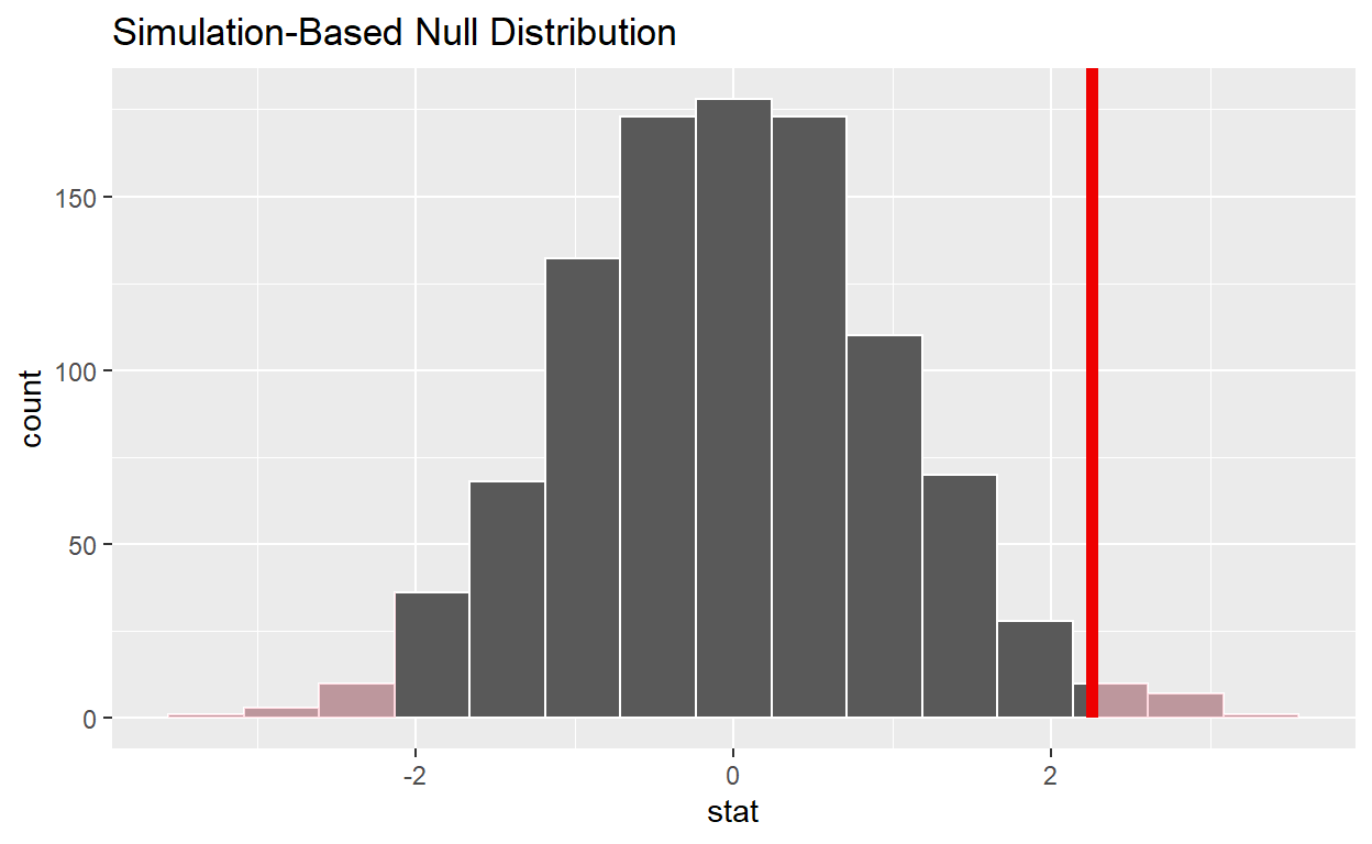
Is the p-value < 0.05? yes
Does your analysis support the null hypothesis that the true mean number of hours worked was 48? no
Question: 2 sample t-test
Make sure you have installed and loaded the tidyverse, infer, and skimr packages
Fill in the blanks
Put the command you use in the Rchunks in your Rmd file for this quiz.
The data this quiz is a subset of HR
- Look at the variable definitions
- Note that the variables evaluation and salary have been recoded to be represented as words instead of numbers
hr_1_tidy.csv is the name of your data subset
- Read it into and assign to
hr_2- Note: col_types = “fddfff” defines the column types factor-double-double-factor-factor-factor
hr_2 <- read_csv("https://estanny.com/static/week13/data/hr_1_tidy.csv",
             col_types = "fddfff")
IS the average number of hours worked the same for both genders in hr_2?
use
skimto summarize the data inhr_2bygenderTable 2: Data summary Name Piped data Number of rows 500 Number of columns 6 _______________________ Column type frequency: factor 3 numeric 2 ________________________ Group variables gender Variable type: factor
skim_variable gender n_missing complete_rate ordered n_unique top_counts evaluation female 0 1 FALSE 4 fai: 81, bad: 71, ver: 57, goo: 51 evaluation male 0 1 FALSE 4 bad: 82, fai: 61, goo: 55, ver: 42 salary female 0 1 FALSE 6 lev: 54, lev: 50, lev: 44, lev: 41 salary male 0 1 FALSE 6 lev: 52, lev: 47, lev: 46, lev: 39 status female 0 1 FALSE 3 fir: 96, pro: 87, ok: 77 status male 0 1 FALSE 3 fir: 89, ok: 76, pro: 75 Variable type: numeric
skim_variable gender n_missing complete_rate mean sd p0 p25 p50 p75 p100 hist age female 0 1 41.78 11.50 20.5 32.15 42.35 51.62 59.9 ▆▅▇▆▇ age male 0 1 39.32 11.55 20.2 28.70 38.55 49.52 59.7 ▇▇▆▇▆ hours female 0 1 50.32 13.23 35.0 38.38 47.80 60.40 79.7 ▇▃▃▂▂ hours male 0 1 48.24 12.95 35.0 37.00 42.40 57.00 78.1 ▇▂▂▁▂
Use
geom_boxplotto plot distributions of hours worked by genderhr_2 %>% ggplot(aes(x = gender, y = hours)) + geom_boxplot()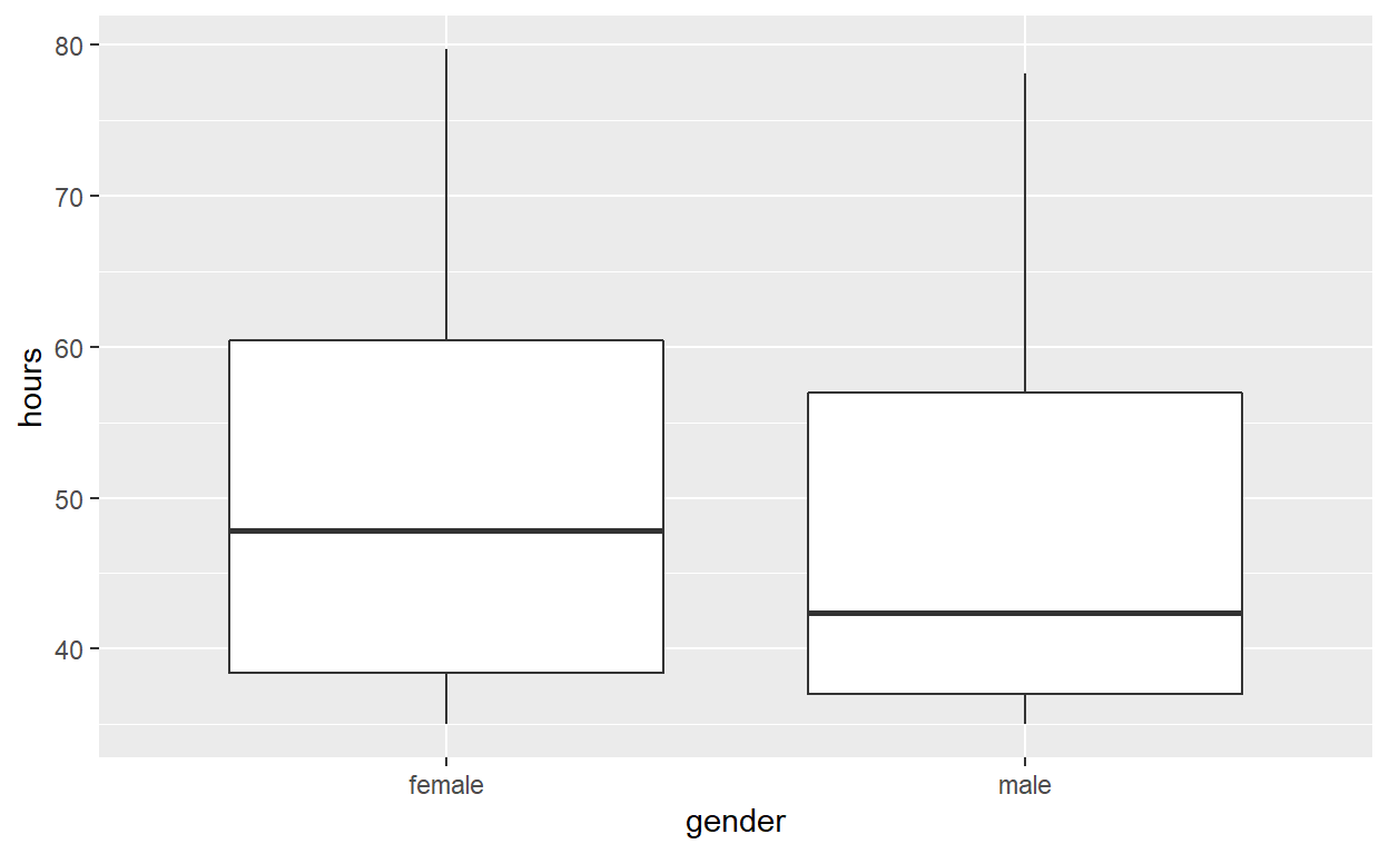
specifythe variables of interest arehoursandgenderResponse: hours (numeric) Explanatory: gender (factor) # A tibble: 500 x 2 hours gender <dbl> <fct> 1 36.5 female 2 55.8 female 3 35 male 4 52 female 5 35.1 male 6 36.3 female 7 40.1 female 8 42.7 female 9 66.6 male 10 35.5 male # ... with 490 more rows
hypothesizethat the number of hours worked and gender are independenthr_2 %>% specify(response = hours, explanatory = gender) %>% hypothesise(null = "independence")Response: hours (numeric) Explanatory: gender (factor) Null Hypothesis: independence # A tibble: 500 x 2 hours gender <dbl> <fct> 1 36.5 female 2 55.8 female 3 35 male 4 52 female 5 35.1 male 6 36.3 female 7 40.1 female 8 42.7 female 9 66.6 male 10 35.5 male # ... with 490 more rows
generate1000 replicates representing the null hypothesishr_2 %>% specify(response = hours, explanatory = gender) %>% hypothesise(null = "independence") %>% generate(reps = 1000, type = "permute")Response: hours (numeric) Explanatory: gender (factor) Null Hypothesis: independence # A tibble: 500,000 x 3 # Groups: replicate [1,000] hours gender replicate <dbl> <fct> <int> 1 36.4 female 1 2 35.8 female 1 3 35.6 male 1 4 39.6 female 1 5 35.8 male 1 6 55.8 female 1 7 63.8 female 1 8 40.3 female 1 9 56.5 male 1 10 50.1 male 1 # ... with 499,990 more rows
Calculatethe distribution of statistics from teh generated data- Assign the output
null_distribution_2_sample_permute - Display
null_dsitribution_2_sample_permute
null_distribution_2_sample_permute <- hr_2 %>%
  specify(response = hours, explanatory = gender) %>%
  hypothesize(null = "independence") %>%
  generate(reps = 1000, type = "permute") %>%
  calculate(stat = "t", order = c("female","male"))

null_distribution_2_sample_permute
Response: hours (numeric) Explanatory: gender (factor) Null Hypothesis: independence # A tibble: 1,000 x 2 replicate stat <int> <dbl> 1 1 -0.208 2 2 -0.328 3 3 -2.28 4 4 0.528 5 5 1.60 6 6 0.795 7 7 1.24 8 8 -3.31 9 9 0.517 10 10 0.949 # ... with 990 more rows
Visualizethe simulated null distributionvisualize(null_distribution_2_sample_permute)
calculatethe statistic from your observed dataAssign the output
observed_t_2_sample_statdisplay
observed_t_2_sample_stat
observed_t_2_sample_stat <- hr_2 %>%
  specify(response = hours, explanatory = gender) %>%
  calculate(stat = "t", order = c("female", "male"))

observed_t_2_sample_stat
Response: hours (numeric) Explanatory: gender (factor) # A tibble: 1 x 1 stat <dbl> 1 1.78
get_p_value from the simulated null distribution and the observed statistic
null_t_distribution %>%
  get_p_value(obs_stat = observed_t_2_sample_stat, direction = "two-sided")
# A tibble: 1 x 1 p_value <dbl> 1 0.072shade_p_valueon the simulated null distributionnull_t_distribution %>% visualize() + shade_p_value(obs_stat = observed_t_2_sample_stat, direction = "two-sided")
Question 3 is the average number of hours worked the same for all three status (fired, ok, and promoted)?
Make sure you have installed and loaded the tidyverse, infer, and skimr packages
Fill in the blanks
Put the command you use in the Rchunks in your Rmd file for this quiz.
The data this quiz is a subset of HR
- Look at the variable definitions
- Note that the variables evaluation and salary have been recoded to be represented as words instead of numbers
hr_2_tidy_csv is the name of your data subset * Read it into and assign to
hr_anova* Note: col-types = fddfff” defines the column types factor-double-double-factor-factor-factorhr_anova <- read_csv("https://estanny.com/static/week13/data/hr_2_tidy.csv", col_types="fddfff")
use
skimto summarize the data inhr_anovabystatusTable 3: Data summary Name Piped data Number of rows 500 Number of columns 6 _______________________ Column type frequency: factor 3 numeric 2 ________________________ Group variables status Variable type: factor
skim_variable status n_missing complete_rate ordered n_unique top_counts gender promoted 0 1 FALSE 2 mal: 90, fem: 89 gender fired 0 1 FALSE 2 fem: 101, mal: 93 gender ok 0 1 FALSE 2 mal: 73, fem: 54 evaluation promoted 0 1 FALSE 4 goo: 70, ver: 62, fai: 24, bad: 23 evaluation fired 0 1 FALSE 4 bad: 78, fai: 72, goo: 25, ver: 19 evaluation ok 0 1 FALSE 4 bad: 53, fai: 46, ver: 15, goo: 13 salary promoted 0 1 FALSE 6 lev: 42, lev: 42, lev: 39, lev: 34 salary fired 0 1 FALSE 6 lev: 54, lev: 44, lev: 34, lev: 24 salary ok 0 1 FALSE 6 lev: 32, lev: 31, lev: 26, lev: 19 Variable type: numeric
skim_variable status n_missing complete_rate mean sd p0 p25 p50 p75 p100 hist age promoted 0 1 40.63 11.25 20.4 30.75 41.10 50.25 59.9 ▆▇▇▇▇ age fired 0 1 40.03 11.53 20.3 29.45 40.40 50.08 59.9 ▇▅▇▆▆ age ok 0 1 38.50 11.98 20.3 28.15 38.70 49.45 59.9 ▇▆▅▅▆ hours promoted 0 1 59.21 12.66 35.0 49.75 58.90 70.65 79.9 ▅▆▇▇▇ hours fired 0 1 41.67 8.37 35.0 36.10 38.45 43.40 77.7 ▇▂▁▁▁ hours ok 0 1 47.35 10.86 35.0 37.10 45.70 54.50 78.9 ▇▅▃▂▁ Employees that were fired worked an average of 41.66959 hours per week.
Employees that were ok worked an average of 47.35118 hours per week.
Employees that were promoted worked an average of 59.20950 hours per week.
Use
geom_boxplotto plot distributions of hours worked by statushr_anova %>% ggplot(aes(x = status, y = hours)) + geom_boxplot()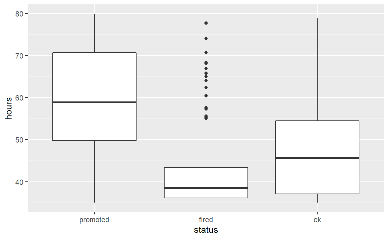
specifythe variables of interest arehoursandstatusResponse: hours (numeric) Explanatory: status (factor) # A tibble: 500 x 2 hours status <dbl> <fct> 1 78.1 promoted 2 35.1 fired 3 36.9 fired 4 38.5 fired 5 36.1 fired 6 78.1 promoted 7 76 promoted 8 35.6 fired 9 35.6 ok 10 56.8 promoted # ... with 490 more rows
hypothesizethat the number of hours worked and status are independenthr_anova %>% specify(response = hours, explanatory = status) %>% hypothesize(null = "independence")Response: hours (numeric) Explanatory: status (factor) Null Hypothesis: independence # A tibble: 500 x 2 hours status <dbl> <fct> 1 78.1 promoted 2 35.1 fired 3 36.9 fired 4 38.5 fired 5 36.1 fired 6 78.1 promoted 7 76 promoted 8 35.6 fired 9 35.6 ok 10 56.8 promoted # ... with 490 more rows
Generate1000 replicates representing the null hypothesishr_anova %>% specify(response = hours, explanatory = status) %>% hypothesize(null = "independence") %>% generate(reps = 1000, type = "permute")Response: hours (numeric) Explanatory: status (factor) Null Hypothesis: independence # A tibble: 500,000 x 3 # Groups: replicate [1,000] hours status replicate <dbl> <fct> <int> 1 41.9 promoted 1 2 36.7 fired 1 3 35 fired 1 4 58.9 fired 1 5 36.1 fired 1 6 39.4 promoted 1 7 54.3 promoted 1 8 59.2 fired 1 9 40.2 ok 1 10 35.3 promoted 1 # ... with 499,990 more rowsThe output has 500000 rows
Calculatethe distribution of statistics from the generated data * Assign the outputnull_distribution_anova* Displaynull_distribution_anovanull_distribution_anova <- hr_anova %>% specify(response = hours, explanatory = status) %>% hypothesize(null = "independence") %>% generate(reps = 1000, type = "permute") %>% calculate(stat = "F") null_distribution_anovaResponse: hours (numeric) Explanatory: status (factor) Null Hypothesis: independence # A tibble: 1,000 x 2 replicate stat <int> <dbl> 1 1 0.312 2 2 2.85 3 3 0.369 4 4 0.142 5 5 0.511 6 6 2.73 7 7 1.06 8 8 0.171 9 9 0.310 10 10 1.11 # ... with 990 more rows
visualize(null_distribution_anova)
calculatethe statistic from your oberserved data * Assign the outputobserved_f_sample_stat * Displayobserved_f_sample_stat`observed_f_sample_stat <- hr_anova %>% specify(response = hours, explanatory = status) %>% calculate(stat = "F") observed_f_sample_statResponse: hours (numeric) Explanatory: status (factor) # A tibble: 1 x 1 stat <dbl> 1 128.
get_p_value from the simulated null distribution and the observed statistic
null_distribution_anova %>%
  get_p_value(obs_stat = observed_f_sample_stat, direction = "greater")
# A tibble: 1 x 1 p_value <dbl> 1 0shade_p_value on the simulated null distribution
null_distribution_anova %>%
  visualize() +
  shade_p_value(obs_stat = observed_f_sample_stat, direction = "greater")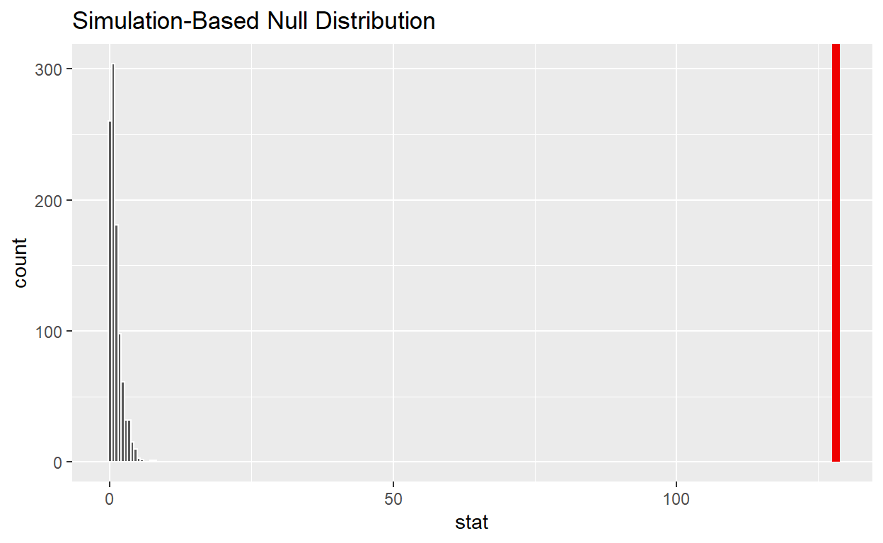
Is the p-value < 0.05? yes
Does your analysis support the null hypothesis that the true means of the number of hours worked for those that were “fired”, “ok” and “promoted” were the same? no
- Assign the output
- Note: col_types = “fddfff” defines the column types factor-double-double-factor-factor-factor
- Read it into and assign to hr